Your First Machine Learning Project (Without Fear)

Machine learning has a reputation for being the deep end of programming: maths-heavy, mysterious, and reserved for people with PhDs. Some of it is. But the core idea is surprisingly ordinary, and with the Python you already know, you can train a real model and use it to make predictions in a few dozen lines. This chapter won’t turn you into a data scientist. What it will do is take the mystery away, so that when you hear people talk about “training a model,” you know exactly what they mean, and you’ve done it yourself.

We’ll start with what machine learning actually does, in plain language, and when it’s the right tool (and, just as importantly, when it isn’t). Then you’ll use a ready-made model from a library, train it, test it honestly, and make predictions. The last part, reading those predictions without fooling yourself, matters more than any of the code.

#What ML actually does

Every program you’ve written so far follows rules that you wrote. If the temperature is above 30, say it’s hot. If the file ends in .jpg, put it in Images. You knew the rules, so you wrote them down.

Now imagine writing the rules for spotting spam email. You might start with “if it mentions a lottery, it’s spam.” Then you’d find legitimate emails about a work lottery, and spam that never uses the word. You’d add more rules, and more exceptions to the rules, and you’d never quite finish, because the pattern is real but too fuzzy to pin down by hand.

Machine learning flips the approach. Instead of writing the rules, you give the computer lots of examples where you already know the answer: thousands of emails, each labelled “spam” or “not spam.” A learning algorithm studies those examples and works out a pattern that connects the email to its label. The result of that learning is called a model. Then, given a new email it has never seen, the model applies the pattern and makes a prediction.

Think about how a child learns to recognise dogs. Nobody gives them a rulebook: four legs, fur, a tail, barks. They see lots of dogs and lots of not-dogs, people tell them which is which, and eventually they just know, even for a breed they’ve never met. Machine learning is a much simpler, more mechanical version of that.

There’s a small vocabulary worth knowing, and you’ll see all of it in our project:

#When ML is useful (and when it isn’t)

Machine learning is powerful, and it’s also over-used. Before reaching for it, it’s worth asking a few honest questions.

Is there a simple rule that works? If you can write the logic as an if statement, write the if statement. Calculating tax, checking a password, sorting files by type: these have exact rules, and a model would only make them slower, harder to understand, and occasionally wrong.

Do you have examples, with answers? A model can only learn from data. For our kind of learning, called supervised learning, you need plenty of examples where you already know the label. A few dozen is rarely enough. Hundreds or thousands is more typical.

Is there actually a pattern? If the features genuinely have nothing to do with the label, no algorithm will find a connection, though some will happily pretend to.

Can you live with mistakes? Every model gets some predictions wrong. That’s fine for suggesting a film or flagging possible spam for a human to check. It’s not fine if a wrong answer costs someone a job, a loan, or their health, unless a person reviews the decision.

Could the answer be hiding in the data? Zara, a graduate analyst at an insurance company, trained her first model to predict which claims would turn out to be fraudulent. It was 99% accurate on the test data, and she was thrilled for about an hour. Then a senior colleague asked which columns she’d used. One of them was investigation_outcome, filled in only after a claim had been investigated. The model hadn’t learned to spot fraud; it had learned to read the answer. With that column removed, accuracy fell to a far more believable 71%. Data scientists call this leakage, and the rule that prevents it is simple: only give a model information you would really have at the moment it has to make its prediction. If a result looks too good to be true, check this first.

So when is machine learning worth using? When there’s a real pattern but it’s fuzzy, when you’ve got plenty of examples to learn from, and when the odd mistake won’t hurt anyone. Spotting objects in photos, estimating house prices, recommending products and guessing which customers might cancel a subscription all fit. It’s a poor fit when you need exact answers, when you’ve only got a handful of examples, or when the decision matters too much to hand over to a pattern nobody can fully explain.

#Using pre-built models safely

You won’t write a learning algorithm from scratch. Almost nobody does for everyday work. Instead you’ll use scikit-learn, the most popular Python library for classic machine learning. It has dozens of ready-made, well-tested algorithms, and they all work the same way: create a model, fit() it to your examples, then predict() on new ones. Install it in your project’s virtual environment:

pip install scikit-learn

(It’s installed as scikit-learn but imported as sklearn.) scikit-learn also installs NumPy, a library for fast number crunching that almost all data work in Python is built on. We’ll use a little of it to create our practice data.

There are also pre-trained models, which someone else has already trained on huge amounts of data. Some recognise thousands of kinds of objects in photos; others transcribe speech, translate between languages or write text. You can download many of them, or use them through an API, much like the weather service in Chapter 19. They can be astonishingly good. They also come with the same responsibilities as anything else you build on.

Whichever kind you use, your own or someone else’s, a few habits will keep you out of trouble.

Always test on data the model hasn’t seen. A model can memorise its training examples, score brilliantly on them and be useless on anything new. Think of the student who memorised last year’s exam answers: full marks on that paper, lost on this year’s. That’s why our project keeps some data back for testing.

Compare with a dumb baseline. If 90% of emails aren’t spam, a “model” that always says “not spam” is 90% accurate and completely useless. So always ask how well the simplest possible guess would do, and make sure your model does better.

Remember that a model learns whatever is in the data, including its unfairness: If past decisions were biased, a model trained on them will be biased too, and it will apply that bias consistently, at scale, with an air of mathematical authority. Be very careful about models that make decisions about people.

Be careful with personal data: Training data about real people needs the same care as any other private information.

Only load saved models from sources you trust: Models are often saved with Python’s pickle system (or joblib, which builds on it). Loading such a file can run code hidden inside it, so a model file from a stranger is as risky as running a stranger’s program.

#Training a simple model

Let’s build a model that predicts whether a student will pass an exam, based on two features: hours of study per week and class attendance. Real student data is private, so we’ll generate made-up data with a hidden pattern built in. More study and better attendance make passing more likely, but there’s luck involved, as there is in real life. This script creates two hundred students:

1# make_students.py - create made-up exam data to learn from
2import csv
3from pathlib import Path
4
5import numpy as np
6
7rng = np.random.default_rng(42)          # same data every time
8count = 200
9hours = rng.uniform(0, 12, count).round(1)
10attendance = rng.uniform(40, 100, count).round()
11
12# the hidden "truth": study and attendance help, with luck mixed in
13chance = 1 / (1 + np.exp(-(0.7 * hours + 0.06 * attendance - 8)))
14passed = (rng.uniform(0, 1, count) < chance).astype(int)
15
16path = Path(__file__).parent / "students.csv"
17with open(path, "w", newline="", encoding="utf-8") as file:
18    writer = csv.writer(file)
19    writer.writerow(["hours", "attendance", "passed"])
20    writer.writerows(zip(hours, attendance, passed))
21print(f"Wrote {count} students to {path.name}")

You don’t need to follow every line of the NumPy here. rng.uniform(0, 12, count) makes 200 random numbers between 0 and 12, all at once. The chance line turns each student’s habits into a probability of passing, and the passed line flips a weighted coin for each student, giving 1 for a pass and 0 for a fail. The fixed seed of 42 means your data will be identical to ours. The first few rows of students.csv look like this:

hours,attendance,passed
9.3,87.0,1
5.3,98.0,0
10.3,70.0,1

Notice the second student: nearly perfect attendance and a decent amount of study, but a fail. Bad luck, a bad day, who knows. Real data is like that, and it’s why no model will be perfect.

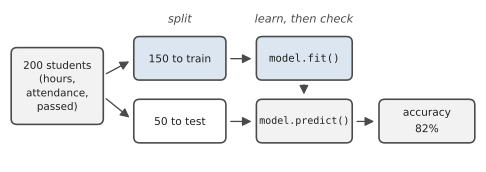
Here’s the plan for training, shown in Figure 26.1. We split the students into two groups. The model learns from 150 of them. The other 50 are kept hidden, and afterwards we see how well the model predicts their results. Those 50 are our honest exam.

#Making and interpreting predictions

Here’s the whole project, pass_predictor.py:

1# pass_predictor.py - predict exam results from study habits
2import csv
3from pathlib import Path
4
5from sklearn.linear_model import LogisticRegression
6from sklearn.metrics import accuracy_score, confusion_matrix
7from sklearn.model_selection import train_test_split
8
9HERE = Path(__file__).parent
10
11
12def load_students(path):
13    features, labels = [], []
14    with open(path, newline="", encoding="utf-8") as file:
15        for row in csv.DictReader(file):
16            features.append([float(row["hours"]),
17                             float(row["attendance"])])
18            labels.append(int(row["passed"]))
19    return features, labels
20
21
22def main():
23    X, y = load_students(HERE / "students.csv")
24    X_train, X_test, y_train, y_test = train_test_split(
25        X, y, test_size=0.25, random_state=0)
26    print(f"{len(X_train)} students to learn from, "
27          f"{len(X_test)} kept back for testing")
28
29    model = LogisticRegression()
30    model.fit(X_train, y_train)
31
32    predictions = model.predict(X_test)
33    accuracy = accuracy_score(y_test, predictions)
34    baseline = max(y_test.count(0), y_test.count(1)) / len(y_test)
35    print(f"Model accuracy on unseen students: {accuracy:.0%}")
36    print(f"Always guessing the most common result: {baseline:.0%}")
37
38    tn, fp, fn, tp = confusion_matrix(y_test, predictions).ravel()
39    print(f"Correct passes: {tp}, correct fails: {tn}")
40    print(f"Said pass but failed: {fp}, said fail but passed: {fn}")
41
42    new_students = {"Sara": [8.0, 90], "Omar": [2.5, 60],
43                    "Lin": [5.0, 75]}
44    print("\nPredictions for new students:")
45    for name, habits in new_students.items():
46        chance = model.predict_proba([habits])[0][1]
47        hours, attend = habits
48        print(f"  {name:<5} {hours:>4} h/week, {attend:>3.0f}% "
49              f"attendance -> {chance:.0%} chance of passing")
50
51
52if __name__ == "__main__":
53    main()

The shape is familiar: load the data, then do things with it. By tradition, the features are called X (a list of lists, one inner list per student) and the labels y (one 0 or 1 per student).

train_test_split() shuffles the students and divides them, keeping 25% back for testing. random_state=0 fixes the shuffle so your results match ours. It returns four lists: features and labels for training, and features and labels for testing.

The model itself is a logistic regression. Despite the name, it’s used for yes-or-no questions like ours. You don’t need the maths behind it to use it well; what it does is find the straight line through the data that best separates passes from fails, and turn each student’s distance from that line into a probability. model.fit(X_train, y_train) is the training step: the model looks at 150 students and their results and learns. That one line is where the machine learning happens.

Run make_students.py once, then the predictor:

150 students to learn from, 50 kept back for testing
Model accuracy on unseen students: 82%
Always guessing the most common result: 62%
Correct passes: 24, correct fails: 17
Said pass but failed: 2, said fail but passed: 7

Predictions for new students:
  Sara   8.0 h/week,  90% attendance -> 93% chance of passing
  Omar   2.5 h/week,  60% attendance -> 9% chance of passing
  Lin    5.0 h/week,  75% attendance -> 48% chance of passing

Let’s read this carefully, the way a careful data scientist would.

Accuracy: On 50 students the model had never seen, it predicted the result correctly 82% of the time. On its own, that number means very little, so we compare it with the baseline: always guessing the most common result would have been right 62% of the time. Our model is clearly doing better than a lazy guess. It has genuinely learned something.

The kinds of mistakes: The confusion matrix breaks the results down. It got 24 passes and 17 fails right. It predicted a pass for 2 students who actually failed, and a fail for 7 who actually passed. Those two kinds of mistake can matter very differently. If the model were used to decide which students get extra help, the 2 it wrongly thought were safe are the worrying ones, because they’d miss out on help they needed. Accuracy alone hides that.

Probabilities, not certainties: predict_proba() gives the model’s estimated chance of each outcome; [0][1] picks the chance of a pass for our one student. Sara, with good habits, gets 93%. Omar gets 9%. And Lin, right in the middle, gets 48%: the model is essentially saying “could go either way.” That honesty is valuable. A good program built on a model should treat a 48% very differently from a 93%.

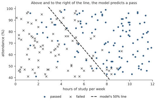
Figure 26.2 shows what the model learned. Each dot or cross is one student. The dashed line is where the model’s estimated chance is exactly 50%. Students above and to the right of it get predicted passes; below and to the left, fails. You can see the crosses on the “pass” side and the dots on the “fail” side. Those are the students luck didn’t follow, and no straight line could have got them all right.

There’s one more lesson hiding here, and it’s the most important one in this chapter. The model found that study and attendance go along with passing. In this case we know that’s genuinely cause and effect, because we built the data that way. But with real data, a model only ever finds patterns, not causes. If ice-cream sales and sunburn rise together, a model will happily use one to predict the other, even though neither causes the other; summer causes both. Models are excellent at spotting what goes together. Working out why is still a job for humans.

#Project: Beginner-Friendly ML Project

You’ve already built the core of the project: a model trained on real (if made-up) data, tested honestly against a baseline, with its mistakes broken down and its predictions given as probabilities. Let’s finish it the way real projects are finished, by saving the trained model so other programs can use it without retraining.

Add this to the end of main():

1    import joblib
2    joblib.dump(model, HERE / "pass_model.joblib")
3    print("Model saved to pass_model.joblib")

joblib comes with scikit-learn, and dump() saves the trained model to a file. Now a completely separate program can load it and make predictions instantly:

1# use_model.py - load the saved model and predict
2from pathlib import Path
3
4import joblib
5
6model = joblib.load(Path(__file__).parent / "pass_model.joblib")
7hours = float(input("Hours of study per week: "))
8attendance = float(input("Attendance (%): "))
9chance = model.predict_proba([[hours, attendance]])[0][1]
10print(f"Estimated chance of passing: {chance:.0%}")

Remember the warning from earlier: only ever load model files you made yourself or got from a source you trust, because loading one can run code.

With this, you have the full life cycle of a machine learning project in miniature: get data, split it, train, evaluate honestly, interpret carefully, save, and reuse. Real projects are bigger, with more data, more features, more careful evaluation, but they have exactly this shape.

Here are some experiments worth trying, each of which teaches something real:

You’ve now taken first steps into the two most exciting areas of modern Python, the web and machine learning. Before we talk about where to go from here, there’s one promise left to keep. The title of this book says automate everyday tasks, and the next three chapters are a collection of ready-to-use automation recipes: email, photos, PDFs, spreadsheets, websites and backups, the jobs people most often wish a computer would just do for them.

#On the Job

How it shows up at work: Machine learning jobs are some of the most talked-about in technology, but most day-to-day ML work is less glamorous than it sounds: finding and cleaning data (everything from Chapters 15 and 20), choosing sensible features, training simple models, and checking honestly whether they’re any good. Many companies also need people who can use models well without building them: plugging a prediction into a report, a web app or a pipeline, and explaining its limits to the people who’ll rely on it.

What employers expect: For a beginner, the honest fundamentals: split the data into training and test sets, measure on data the model hasn’t seen, look beyond accuracy at the kinds of mistakes, and compare against a simple baseline. Know the scikit-learn pattern of fit, predict and predict_proba. Know what overfitting and leakage are. Above all, be able to explain a model’s results and limitations to someone who isn’t technical.

Interview questions you might meet:

Portfolio task: Push the pass predictor, and in the README, write a short “Limitations” section: what data it was trained on, how accurate it is on unseen students, what kinds of mistakes it makes, and what it should not be used for. A plain-English limitations section is something many professional projects lack, and it shows maturity.

Professional habit: Before training any model, write down the simplest possible baseline (always predict the most common answer, or a one-line rule) and its score. A model is only interesting if it beats that.

#Exercises

Solutions are in solutions/chapter_26 in the book’s GitHub repository, along with a copy of students.csv. They need scikit-learn, installed as described in this chapter.

Warm-up

Practice

Challenge